INTRODUCTION
Large Language Models (LLMs) have rapidly evolved to become powerful tools for a wide range of natural language processing tasks, including question answering, summarization, and reasoning.
Despite their impressive generative abilities, a critical limitation of current LLMs lies in their uncertainty and lack of calibrated confidence in generated outputs. These models often produce fluent but incorrect or misleading responses, a phenomenon commonly referred to as hallucination [1]. As LLMs are increasingly deployed in decision-critical applications such as procurement analytics, finance, and healthcare, estimating the confidence and factual reliability of their outputs becomes essential.
Traditional approaches to model confidence estimation in machine learning typically rely on probabilistic measures derived from model outputs, such as SoftMax probabilities or entropy [2] [3]. However, for autoregressive language models, token-level probabilities only partially capture uncertainty [4], since contextual coherence, semantic stability, and factual correctness are not explicitly modeled [5]. To address these challenges, recent research has explored multiple complementary directions: analyzing token probability distributions [2] [3], evaluating self-consistency [6] across multiple generations, and using embedding similarity [7] [8] to capture semantic agreement between responses.
We propose a unified framework for estimating LLM output confidence. It extracts intrinsic features, including token probabilities, minimum token probability, token entropy, and self-assessment scores, and measures self-consistency via multiple responses per query, computing the mean and variance of inter-response correlations and cluster similarities. These features are then used to train a Random Forest model with LLM-as-Judge [9] as the target, which independently evaluates factual correctness, hallucination, and faithfulness against ground-truth references.
We evaluate our framework using two datasets of differing complexity and domain characteristics: a subset of the Open Trivia dataset [10], representing general knowledge tasks, and an expert-annotated procurement dataset, representing a specialized, real-world domain. Experiments were conducted on two models: the Llama-3.2-1B-Instruct model (hereafter referred to as the "base model" throughout this paper) [11] and a Llama-3.2-1B-Instruct model fine-tuned using Parameter-Efficient Fine-Tuning [12] on procurement data (hereafter referred to as the "fine-tuned model" throughout this paper). Finally, we perform statistical tests and quantify the stability of feature importances of the intrinsic features across various model-data combinations.
This integrated approach aims to move beyond traditional probability-based uncertainty estimation, offering a more holistic understanding of how confident an LLM truly is in its generated outputs and the weights of the factors and their stability that decide confidence across various model-data configurations.
LITERATURE SURVEY
Probabilistic/token-level confidence and calibration:
A classical and widely used approach to model confidence relies on probabilities of output by the model and on information-theoretic summaries such as entropy. [9] showed that modern neural networks are often poorly calibrated and proposed temperature scaling as a simple post-hoc fix for classification models; their work established Expected Calibration Error (ECE) and similar diagnostics as standard tools for calibration analysis. Recent work has extended calibration analysis specifically to LLMs [13] [14], showing that alignment steps (e.g., reinforcement learning with human feedback) and model size/architecture can substantially change calibration behavior and that generation/factuality calibration is an active area of research. Several recent studies propose token-level uncertainty measures (e.g., per-token entropy, length-normalized entropy, minimum token probability, and perplexity-based scores) [15] and show they can be useful for spotting low-confidence or potentially incorrect spans but also note caveats (response length effects, tokenization artifacts, and the fact that high fluency does not guarantee factuality). Key points/methods to note:
1. Token probabilities & entropy. Computing the conditional distribution over the next token and summarizing it (mean token entropy, max/min token probability, joint/sequence entropy, or length-normalized entropy) [16] is a straightforward white-box measure when you have access to logits/probabilities. Several recent papers formalize token-level uncertainty estimation and show its utility for flagging suspicious tokens and segments [16] [17].
2. Calibration diagnostics. ECE and reliability diagrams remain common tools to evaluate whether reported probabilities reflect empirical correctness; for LLMs, new work investigates calibration across generation, factuality, and multiple-choice questions and how alignment affects calibration [18].
Self-consistency and embedding-based stability
Researchers have used multiple-sample decoding [19] to assess whether a model consistently returns the same (or semantically similar) answer under sampling or diverse decoding. The self-consistency decoding strategy [20] was proposed in the context of chain-of-thought reasoning: sample many reasoning paths and select the most consistent answer by marginalizing across samples, a technique that improves reasoning performance and provides an implicit consistency signal. Measuring semantic similarity between multiple outputs commonly uses sentence/response embeddings [21] and cosine similarity or correlation-based summaries (mean pairwise cosine, mean inter-response correlation) to quantify stability across runs. These embedding-based stability measures are widely used for paraphrase detection, ensemble agreement scoring, and response deduplication.
Clustering of embeddings and cluster-based similarity scores
Clustering model output embeddings to discover modes (distinct answer clusters), then summarizing cluster compactness or cluster similarity as a measure of coherence, has become an effective way to capture multi-modal behavior of LLM outputs [22]. Work on using embeddings from large models for text clustering documents that LLM embeddings often produce semantically meaningful clusters and that cluster cohesion/separation metrics (e.g., silhouette, intra-cluster cosine similarity) can be interpreted as a proxy for semantic agreement across responses. Recent papers [23] explore best practices for clustering LLM embeddings and stress preprocessing choices (embedding model, normalization, clustering algorithm, number of clusters) as having large effects on the resulting metrics.
LLM-as-Judge, factuality checking, hallucination, and faithfulness metrics
Using LLMs themselves to judge [24] [25] or score other model outputs has gained rapid traction (industry and research). Seminal and influential frameworks for LLM-as-Judge / LLM-based evaluation include G-Eval (using GPT-4o with chain-of-thought and form-filling for robust subjective scoring) and GPTScore (a general framework for scoring generated text with LLMs) [26]. Larger surveys and focused studies examine the strengths and failure modes of this approach.
LLM judges scale cheaply compared to human annotation and can produce multi-aspect, promptable assessments (e.g., correctness, hallucination, faithfulness), but they can also exhibit bias (e.g., preferring outputs similar to their own training distribution) [27] and must be meta-evaluated against human judgments. There are also many model-based factuality methods (QAGS [28], FactCC [29]) that either generate questions based on candidate text or check atomic claims with external evidence. Studies of hallucination [30] laid out the groundwork by categorizing hallucination types and evaluating summarization models’ faithfulness.
Hallucination, faithfulness, and the limits of single-metric evaluation
A recurring theme in the literature is that no single metric perfectly captures trustworthiness [31]. Token-probability measures are sensitive to surface form and tokenization; embedding-based measures capture semantic similarity but not factual correctness, and LLM judges can be powerful but show biases and require meta-evaluation. [32] articulated the prevalence of hallucinations in abstractive summarization and categorized types of hallucinated content; [33] and [34] proposed automated protocols that better detect factual inconsistency than traditional lexical overlap metrics.
Surveys and meta-evaluations (LLM-as-Judge & UQ)
There are recent survey, and meta-analysis works that summarize the LLM-as-Judge paradigm and the space of uncertainty quantification (UQ) techniques for LLMs. These works are useful to position a multi-signal confidence estimation pipeline and to identify best practices and pitfalls, including the need for meta-evaluation against human labels or external evidence [35].
Gaps, open challenges
While these approaches perform reasonably well for specific model-data combinations, systematic investigation of how the metrics and their relative importances are affected by fine-tuning and domain-specific data remains limited. Additionally, relying on LLM-as-Judge necessitates a third-party model to validate results, which introduces privacy constraints and additional computational overhead.
METHODOLOGY
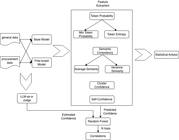
To evaluate confidence estimation methods for LLMs (base and fine-tuned) in the general and procurement domains, we designed a systematic study combining intrinsic and extrinsic confidence measures. This section details the models, dataset, evaluation metrics, and experimental setup used in our analysis. Figure 1 provides an overview of the feature extraction pipeline, illustrating how model outputs are generated, transformed into token-level and semantic features, and aggregated for downstream analysis. First, multiple outputs are generated from each model for every query. Second, several features like token-level probability, entropy features, semantic consistency, and self-confidence scores are computed directly from the model logits and output. Then we perform detailed statistical analysis on the feature importances of the extracted features.
Models and Rationale
We used two instruction-tuned models from the LLaMA 3.2 family:
1. Llama-3.2-1B-Instruct (Base) - a compact model with 1 billion parameters, optimized for efficiency.
2. Llama-3.2-1B-Instruct-finetuned (Fine-tuned) - a mid-scale model with 1 billion parameters, which was fine-tuned on procurement data.
The fine-tuned model provides higher fluency and reasoning capacity on procurement data compared to the base model. Llama-3.2-1B-Instruct is a suitable choice for this study because it provides a compact, instruction-tuned architecture that is both computationally efficient and sufficiently expressive for controlled confidence-estimation experiments. Its small parameter count allows feature extraction and fine-grained uncertainty analysis at scale without prohibitive cost. Moreover, its open-weights nature facilitates domain-specific fine-tuning; when adapted to procurement data, the model can better internalize domain terminology and reasoning patterns, enabling more realistic evaluation of confidence signals within a specialized application setting.
Details of fine-tuning
The Llama 3.2 model was fine-tuned using the Unsloth framework [36] with supervised instruction tuning to adapt it for domain-specific question-answering tasks in strategic procurement and supplier management. The pre-trained unsloth/Llama-3.2-1B-Instruct model and its tokenizer were initialized with a chat template following the Llama-3.1 conversational format [37]. The dataset was preprocessed into user-assistant dialogue pairs to align with the model’s instruction-following format. Fine-tuning was conducted using the SFTTrainer from the TRL library [38] with mixed-precision training and 4-bit quantization [39] to optimize computational efficiency. The optimization process used the Adam optimizer [40], linear learning rate scheduling, and gradient accumulation to ensure stable convergence. An early stop ping mechanism monitored evaluation loss to mitigate overfitting, while only assistant responses were included in gradient updates to refine model generation quality. This fine-tuning strategy enabled the model to internalize the specialized communication patterns and analytical reasoning required for procurement strategy assistance.
Both models were selected to represent resource-constrained but practically deployable LLMs for procurement use cases, where organizations may not have access to larger commercial systems.
Dataset
We evaluate the models on two types of datasets.
General knowledge data – TriviaQA subset
From the full TriviaQA dataset [10] (~95K question-answer pairs with supporting evidence), we randomly sampled 10,000 questions to create a manageable evaluation set. The sampling was uniform across all topics, without any filtering based on question type or difficulty, ensuring that the subset is representative of the overall dataset. However, since this is a subset, rare or highly specialized topics may be underrepresented, slightly reducing the tail-end diversity compared to the full dataset. Overall, the sample maintains broad topical coverage but introduces minor stochastic variability due to random selection.
Question: What was the capital of West Germany?
Answer: Bonn
2. Procurement subset: We curated several hundred queries manually to cover diverse aspects of procurement. The selection was guided by domain coverage: supplier assessment, contract analysis, compliance and regulation, risk identification, and general procurement knowledge. Each category was represented proportionally to reflect typical procurement scenarios encountered in practice. While this approach guarantees domain relevance, it introduces potential bias toward scenarios the curators deemed important and may underrepresent edge cases or less common procurement topics. Sample question and answer below:
Question: How do high-risk and high-value procurement activities differ in processing times from low-risk and low-value activities?
Table 1: The calculated metrics for base/fine-tuned models with procurement/general data. ↑ indicates higher values are better; ↓ indicates lower values are better indicators of confidence.
| Model-Data | Token Prob ↑ | Min Prob ↑ | Entropy (nats) ↓ | Ans Corr ↑ | Faith ↑ | Hal ↑ | Avg Sim ↑ | Cluster Conf ↑ | Self Conf ↑ | Var Sim ↓ |
|---|---|---|---|---|---|---|---|---|---|---|
| Base-Procurement | 0.79 | 0.04 | 2.51 | 0.35 | 0.96 | 0.37 | 0.85 | 0.33 | 7.88 | 0.015 |
| Base-General | 0.78 | 0.12 | 1.93 | 0.35 | 1.00 | 0.31 | 0.70 | 0.33 | 7.90 | 0.028 |
| Fine-tuned-Procurement | 0.55 | 0.01 | 1.60 | 0.49 | 0.97 | 0.40 | 0.83 | 0.20 | 7.19 | 0.004 |
| Fine-tuned-General | 0.62 | 0.07 | 1.56 | 0.30 | 1.00 | 0.25 | 0.68 | 0.25 | 2.89 | 0.018 |
Answer: High-risk and high-value procurements take longer, while low-risk, low-value activities are processed about 30% faster.
Each query was designed to test the models’ ability to provide factual, faithful, and contextually relevant answers.
Implications: These selection processes introduce two types of variability: (1) stochastic variability from random sampling in TriviaQA and (2) systematic variability and potential bias from manual curation in the procurement subset.
EXPERIMENTAL SETUP
Inference Parameters: Both models were run with consistent decoding settings (e.g., temperature = 0.7, top-p = 0.9) to balance fluency and diversity.
Where,
temperature: controls the randomness of token sampling; higher values produce more diverse outputs, while lower values make responses more deterministic.
top-p: limits token selection to the smallest cumulative probability mass p, ensuring sampling only from the most probable subset of tokens.
Hardware Environment:
GPU: NVIDIA GPU with CUDA
RAM: 16GB VRAM
Platform: Google Cloud Platform
Instance Type: g2-standard-8
FEATURE EXTRACTION PIPELINE
1. Query Submission and Output Generation: For each input query, requests are sent to both models under evaluation. Each query is executed multiple times per model (five generations) with a temperature below 1 to encourage diverse yet coherent outputs.
2. Token-Level Probabilities: The model outputs logits, which are transformed into token-level probabilities using the SoftMax function. The token probabilities are calculated using:
pi(T)=exp(zi/T)∑j=0K expzj/T (1)
Where T is the temperature parameter, T=1 is the normal SoftMax, T<1, makes the output more deterministic, T>1 makes the output more random. From these probabilities, we compute:
3. Average Token Probability: Measures how consistently the model selects tokens from a sharp distribution. Higher values indicate more confident token selection.
4. Minimum Token Probability: Captures the lowest-confidence token in the output, highlighting potential weak points in the model’s prediction.
5. Token Entropy: Using the token probabilities, entropy is calculated for each output. High entropy indicates many plausible next tokens (uncertainty), while low entropy reflects a concentrated belief in the chosen tokens.
The entropy is calculated using:
H(T)=-∑iK pi(T)log(pi(T)) (2)
Where, pi(T) is the probability of ith token, T is the temperature parameter and K is the vocabulary size.
6. Semantic Consistency Measures: Each set of five outputs per query is encoded into 384-dimensional embeddings using the pretrained all-MiniLM-L6-v2 model. From these embeddings, we compute:
1. Average Similarity: Mean of the upper-triangular elements of the 5×5 cosine similarity matrix, reflecting the consistency of model outputs.
2. Variance-Similarity: Variance of the upper-triangular elements, quantifying output dispersion across generations.
7. Cluster Confidence: The embeddings are clustered using agglomerative clustering. The Cluster Confidence Score is computed as the ratio of the number of embeddings in the largest cluster to the total embeddings. A higher score indicates that outputs are semantically aligned, while a lower score reflects diverse, potentially unstable outputs.
Self-Confidence Scores:
Table 2: Feature relevance, complements and error sensitivity to model errors
| Feature | Relevance | Complementarity | Error Sensitivity |
|---|---|---|---|
| Average Token Probability/ Minimum Token Probability | Captures the LLM’s internal uncertainty during decoding and are strongly connected to the confidence assigned by the underlying the LLM. | Provides a local view of uncertainty that semantic coherence metrics cannot capture | Particularly sensitive to lexical/syntactic ambiguity, hallucinations and out-of-vocab prompts that flatten the token distribution. |
| Token Entropy | As a distributional measure, it captures uncertainty independently of any specific chosen token. | Entropy complements probability-based features by differentiating between low average probability due to scattered uncertainty versus due to localized uncertainty. | Sensitive to ambiguity, especially when the prompts under-specify information. |
| Average Similarity/ Variance-Similarity | Measures output-space stability rather than token-level certainty, thereby capturing higher-level semantic or conceptual consistency. | Offers a macroscopic view of uncertainty that can reveal semantic drift even when token-level probabilities appear confident | Sensitive to errors driven by ambiguous prompts where different generations diverge semantically. |
| Cluster Confidence | Calculates semantic coherence at a coarser level than pairwise similarity, indicating whether the model converges on one stable interpretation or several competing answers. | Encodes structural variability in the answer space, which average similarity cannot fully characterize. | Particularly sensitive to multi-modal or conflicting interpretations of the prompt, inconsistent reasoning paths that produces distinct answer modes. |
| Self-Confidence Scores | Reflects an introspective signal distinct from token probabilities or semantic variance and often correlates with calibrated judgments of difficulty. | Unlike probabilistic and entropy measures, this captures more semantic information and scores based on this | Particularly sensitive to reasoning errors and factual uncertainty; models often lower their self-score when faced with unclear prompts. |
Each model is re-prompted with the original question and its own generated answer to provide a self-assessment on a 1–10 scale. This score reflects the model’s perceived reliability of its response.
Feature Aggregation:
All extracted features (token-level, semantic, clustering, and self-confidence) are combined into a single feature vector per query for downstream analysis.
The mean values of the calculated metrics for Llama 3.2, the fine-tuned model with procurement data, and the general domain data are presented in Table 1, showing Token Probabilities (Token Prob), Minimum Token Probability (Min Prob), Token Entropy (Entropy), Answer Correctness (Ans Corr), Faithfulness (Faith), Hallucination (Hal), Average Similarity (Avg Sim), Cluster Confidence (Cluster Conf), Self Confidence (Self Conf), and Variance Similarity (Var Sim). As observed, the Answer-Correctness score is higher for the fine-tuned model compared to the base Llama 3.2 model when evaluated on procurement data, indicating the effectiveness of domain-specific fine-tuning. However, a slight decrease in correctness scores is observed when the same fine-tuned model is evaluated on general data, suggesting limited generalization beyond the fine-tuning domain. Additionally, the fine-tuned model exhibits a higher hallucination score (where a greater score corresponds to a lower hallucination tendency), further demonstrating its improved reliability and factual consistency within the procurement domain.
Furthermore, in Table 2, we show how the features are relevant to confidence estimation, how these features complement each other, and which kind of model errors each feature is sensitive to; this provides a clear conceptual foundation for further analysis.
RESULTS
Correlation between the variables
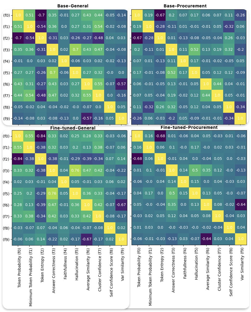
The correlations between the extracted metrics are illustrated in Figure 2, shown
for base/fine-tuned models with general/procurement data. Key observations include:
Similarity of Correlation Matrices
The correlation matrices look similar for both models on general data. This indicates that the fine-tuning process has not changed the model considerably on general data, and the metrics that estimate the confidence scores are consistent.
Difference of Correlation Matrices
On the other hand, the correlation matrices for both models on procurement data look much different, specifically looking at the correlation between Average-Similarity and Variance Similarity, which has a value of 0 for the base model and -0.62 (high negative) for the fine-tuned model, which means the spread/variance of the similarity scores is lesser when the average similarity score is higher. In other words, the fine-tuned model has learned to be more deterministic about where it’s right (small variance when the mean is high) and more exploratory where it’s uncertain (large variance when the mean is small).

Low Correlations
Another notable difference is the relatively low correlation between the average token probabilities and answer correctness for the fine-tuned model on procurement data. This is a strong indication that the probability values are not calibrated well. The authors identify several reasons for this behavior.
1. Fine-tuning with cross-entropy loss on gold-standard responses penalizes incorrect tokens strongly while providing reward only to the exact target token. Consequently, the model minimizes loss most effectively by assigning very high probabilities to the selected tokens, leading to a saturated output distribution that diminishes the variance and weakens the correlation between token probabilities and actual correctness.
Calibration Loss:
We observe that fine-tuning a model results in a loss of probabilistic calibration due to the following reasons:
1. Distribution shifts: Fine-tuning on domain-specific data like procurement data skews the input distribution. Because the model is optimized to fit to a narrower distribution, its output probabilities begin to reflect the loss function it was trained on rather than statistical properties learned during pretraining.
2. Fine-tuning often focuses on next token prediction correctness, rather than well-calibrated likelihoods. This causes the model to over- (or under-) estimate token confidence levels.
3. Training on broad data enforces calibration through diverse linguistic and semantic conditions. However, fine-tuning on limited domain data reduces diversity and consequently the ability of the model to estimate uncertainty.
4. Fine-tuning improved competence specialization (tight clusters where it performs well) but reduced epistemic calibration (token probabilities no longer informative). To address the calibration issue, we use isotonic regression from scikit-learn [39], as shown in Figure 3. The correlation between average token probabilities and answer correctness before and after calibration was 0.007 and 0.15, respectively, indicating an increase in calibration scores for the model.
Entropy and Token Probability:
Entropy exhibits a strong inverse correlation with token probability, consistent with its mathematical definition defined in Equation (2).
LLM-as-Judge Correctness and Hallucination
LLM-as-Judge Correctness shows a weak correlation with token probability and a moderate positive correlation with hallucination scores. This also shows that token probability alone is a bad estimator of LLM correctness.
Average Similarity and Cluster Confidence:
Average-Similarity and Cluster Confidence are strongly correlated with each other, moderately correlated with Answer-Correctness, and weakly correlated with the remaining metrics.
Self-Confidence and Relevancy:
Self-confidence scores demonstrate moderate positive correlations with LLM-as-Judge. Answer-Correctness and entropy, and a moderate inverse correlation with minimum token probability.
Additionally, the mean score of average correctness obtained for the base model was 0.3, whereas the fine-tuned model was 0.49, meaning that the fine-tuned model got more of the procurement questions correct, as noted in Table 1.
Answer-Correctness Prediction using internal features
The internal features refer to metrics derived directly from the model’s own outputs, without the involvement of an external evaluator or an LLM-as-a-Judge. These features include token probability, minimum token probability, entropy, average-similarity, cluster confidence, and self-confidence scores.
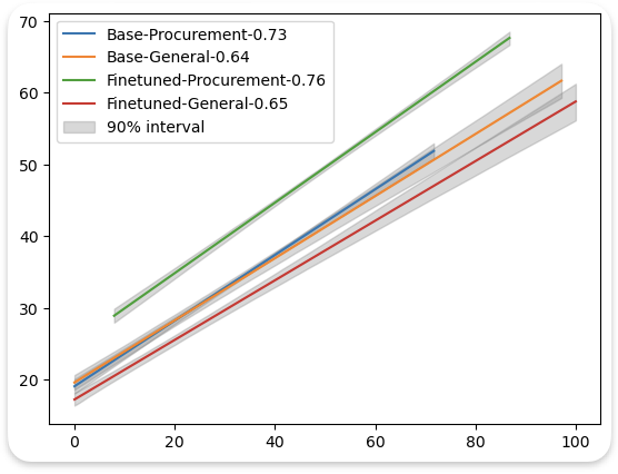
Actual Confidence (%)
Figure 4: Confidence prediction (%) using internal features for base/fine-tuned models on procurement/general data. The legend shows model-data combination with correlation scores with the target.
Table 3: The feature importances for base/fine-tuned models with procurement/general data. Higher values are better.
| Model-Data | Token Probability | Minimum Token Probability | Token Entropy | Cluster Confidence | Average Similarity | Self-Confidence | Variance-Similarity |
|---|---|---|---|---|---|---|---|
| Base-Procurement | 0.11 | 0.11 | 0.09 | 0.02 | 0.21 | 0.11 | 0.33 |
| Base-General | 0.11 | 0.20 | 0.16 | 0.11 | 0.17 | 0.02 | 0.13 |
| Fine-tuned-Procurement | 0.10 | 0.13 | 0.09 | 0.00 | 0.38 | 0.05 | 0.24 |
| Fine-tuned-General | 0.10 | 0.19 | 0.11 | 0.01 | 0.43 | 0.03 | 0.12 |
The core intuition behind predicting the Answer-Correctness score is to eliminate the dependency on third-party models for estimating the confidence of our system’s predictions. To achieve this, we use an ensemble learning approach using Random Forest regression [41], which aggregates predictions from multiple decision tree regressors trained on different sub-samples of the dataset. This ensemble averaging helps to improve predictive accuracy while mitigating overfitting.
We chose the Random Forest model because it is robust to outliers, models non-linear relationships well, and can be trained on very little data, usually better than using a single decision tree. In addition to this, it also provides feature importances. One of the limitations is overfitting, which we overcome by using cross-validation. Also, interpretability becomes hard when using an ensemble; however, interpretation is not the focus of the work presented here.
In our experiments, the target variable is the Answer-Correctness Scores provided by the external LLM, while the input features comprise the internal features listed above. The experiments were conducted on the base model and its fine-tuned variants, trained on both procurement-specific and general-purpose datasets. Cross-validation results demonstrate that the Random Forest model’s predictions show stronger correlations with the ground-truth correctness scores for the fine-tuned model on procurement data (4.1% higher), and performance is slightly better on general data (1.5% higher) (see Figure 4).
In Figure 4, we show the linear trend lines along with a computed 90% confidence interval. The 90% confidence intervals for predicted confidence scores were 2.3 times narrower for models evaluated on domain-specific data compared to those evaluated on general knowledge data. This indicates greater consistency and lower uncertainty in confidence estimation within the domain context, suggesting that domain familiarity enhances the stability of the model’s internal uncertainty representation.
The Random Forest regressor was configured with 100 estimators, a minimum sample split of 2, and minimum samples per leaf of 2, using variance reduction as the splitting criterion. Feature importance analysis (Table 3) reveals that both models assign the greatest importance to Average-Similarity and Variance-Similarity. This is because of the way these features are calculated. Both these features are calculated by taking multiple (five) outputs and calculating the similarity and variance between them. The model that is confident in its output will generate answers that are consistent with each other, resulting in higher similarity scores and lower variance, whereas a model that is not confident will hallucinate more, which results in inconsistent answers in each run, consequently producing lower similarity scores and higher variance. These features are followed by token probability, minimum token probability and token entropy, which are closely related features and provide good heuristics for confidence.
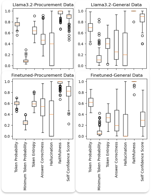
Feature Consistency
We also conducted a feature consistency analysis to evaluate the stability of the computed internal metrics such as token probability, entropy, and related features. Since each query was executed five times, yielding five distinct responses per query, we calculated the mean of each feature across these five responses. Subsequently, we computed summary statistics of these mean values to assess the overall stability of each feature (see Figure 5).
To ensure a fair comparison, all feature metrics were normalized prior to analysis. The results indicate that self-confidence scores, answer correctness, token probabilities scores exhibit greater variability on general data compared to procurement-specific data, which aligns with our expectations given the more diverse nature of general queries. Although fine-tuning on procurement data increased mean answer correctness, the variance in correctness scores also rose slightly. This suggests that fine-tuning improved domain alignment and overall accuracy but also introduced greater sensitivity to input variation within the domain. The effect likely reflects a bias-variance trade-off: fine-tuning enhances specialization and confidence but can reduce the smoothness and calibration consistency of model predictions.
In general, lower variance values correspond to higher feature consistency, implying more stable and reliable model behavior across multiple runs. These findings underscore the importance of consistency analysis when evaluating internal confidence indicators in LLMs.
Features
Figure 5: Feature Consistency
Statistical tests for feature importance
Similar to the feature importances shown in Table 3, we obtain feature importance values for several hundred samples of model-data pairs (i.e., with base/fine-tuned models with general/procurement data) and perform the Kruskal–Wallis Test [42]. This nonparametric test is appropriate because it does not assume normality and compares median ranks across multiple independent groups, making it well-suited for feature importance distributions that may be skewed or non-Gaussian. The results of this test showed extremely small p-values for all features, ranging from 10−24 to 10−55. This is easy to see when analyzing the correlations between the features and the target (answer correctness), although correlation works best on linear data, it still provides important insights on the behavior. We find that the correlation between average-similarity and the target on procurement data for base and fine-tuned models is 0.12 and 0.35 respectively, indicating a higher correlation for the fine-tuned model on procurement data, consequently giving a higher importance and low p-values. We also find that token entropy has a stronger negative correlation with the target on general data (-0.35) than on procurement data (~0) for both models; this arises because the model’s uncertainty signals are more reliable in domains that closely match its pretraining distribution. In contrast, domain-specific data weakens this relationship; thus, we have higher feature importance for entropy on general data than on procurement data, leading to a low p-value. Assuming 𝛼 = 0.05 (significance level), this provides a strong indication that the features are significantly different across at least one model-data configuration.
When the Kruskal–Wallis test indicates a statistically significant overall difference, it does not specify which groups differ. To identify these specific differences, we conduct pairwise Dunn’s tests [43], which compare the mean rank differences between all pairs of groups while maintaining the rank-based, nonparametric framework. Because multiple pairwise comparisons inflate the risk of Type I errors (false positives), we apply a Bonferroni correction [44] to control the family-wise error rate and ensure the reliability of the conclusions. The results of this are shown in Table 4. The p-values less than 𝛼 = 0.05 have been highlighted in bold. The table clearly indicates most features are significantly different across model-data configurations; the only notable exception is Base-General with Base-Procurement for Token Probability, which has a p-value of 1, indicating that the token probabilities are not too different; this is indicative of a well-calibrated model. Whereas token probability p-value for the fine-tuned model is much lower than 𝛼, indicating a less calibrated model.
Table 4: P-Values obtained from post-hoc pairwise Dunn tests with Bonferroni correction
| Model-Data (A) | Model-Data (B) | Token Prob | Min Prob | Entropy | Ans Corr | Cluster Conf | Avg Sim | Self Conf | Var Sim |
|---|---|---|---|---|---|---|---|---|---|
| Base-General | Base-Procurement | 1 | 0 | 0 | 0.004 | 0.1588 | 0.004 | 0 | 0 |
| Base-General | Fine-tuned-General | 0.0057 | 0.7686 | 0.0127 | 0 | 0 | 0 | 0.0099 | 0.0062 |
| Base-General | Fine-tuned-Procurement | 0 | 0 | 0 | 0 | 0.0004 | 0 | 0 | 0.0045 |
| Base-Procurement | Fine-tuned-General | 0.2633 | 0 | 0 | 0.0029 | 0 | 0.0029 | 0 | 0 |
| Base-Procurement | Fine-tuned-Procurement | 0 | 1 | 0.0563 | 0 | 0 | 0 | 0.0028 | 0.005 |
| Fine-tuned-General | Fine-tuned-Procurement | 0.0042 | 0 | 0.0046 | 0.0278 | 0.0155 | 0.0278 | 0.0085 | 0 |
CONCLUSION
This study demonstrates that feature-based methods can effectively estimate confidence in LLMs. Using Llama 3.2 1B-Instruct and its fine-tuned variant, we show that interpretable features capturing response consistency serve as strong predictors of correctness, achieving correlations of 0.65 on procurement-specific data and 0.75 on general data. Token probability and entropy features also contribute meaningfully, though with more moderate influence. However, one of the limitations of this analysis is using LLM-as-Judge, which itself is prone to errors and hallucination. Our analysis helps in designing confidence estimation systems by assigning importances for various features in various circumstances, like fine-tuned and domain-specific data. Our analysis can be extended by testing other LLM architectures like encoder-only, encoder-decoder etc., it is also useful to fine-tune models preserving the calibration. Our approach derives confidence from model-internal signals, which can be informative but are not guaranteed to be well calibrated. Classical methods like conformal prediction derive confidence from external, empirically calibrated error quantiles, providing guaranteed coverage even when the model’s internal uncertainty signals are unreliable. Beyond predictive performance, our analysis reveals that both fine-tuning and domain specialization significantly reshape the feature landscape of confidence estimation. Statistical tests (p < 10⁻²⁴) confirm that most confidence-related features differ across model–data configurations, indicating that model adaptation fundamentally alters how confidence is internally represented. These results highlight that LLM confidence is not a fixed property but a behavior that evolves with data and fine-tuning, and that interpretable feature analysis offers a practical route toward quantifying and understanding this evolution.